Modern Recommendation System Framework
Recommendation
Optimization
matchmaking
- Modern Recommendation System Framework
These systems typically involve documents (entities a system recommends, like movies or videos), queries (information needed to make recommendations, such as user data or location), and embeddings (mappings of queries or documents to a vector space called embedding space).
Below is a common architecture for a recommendation system model:
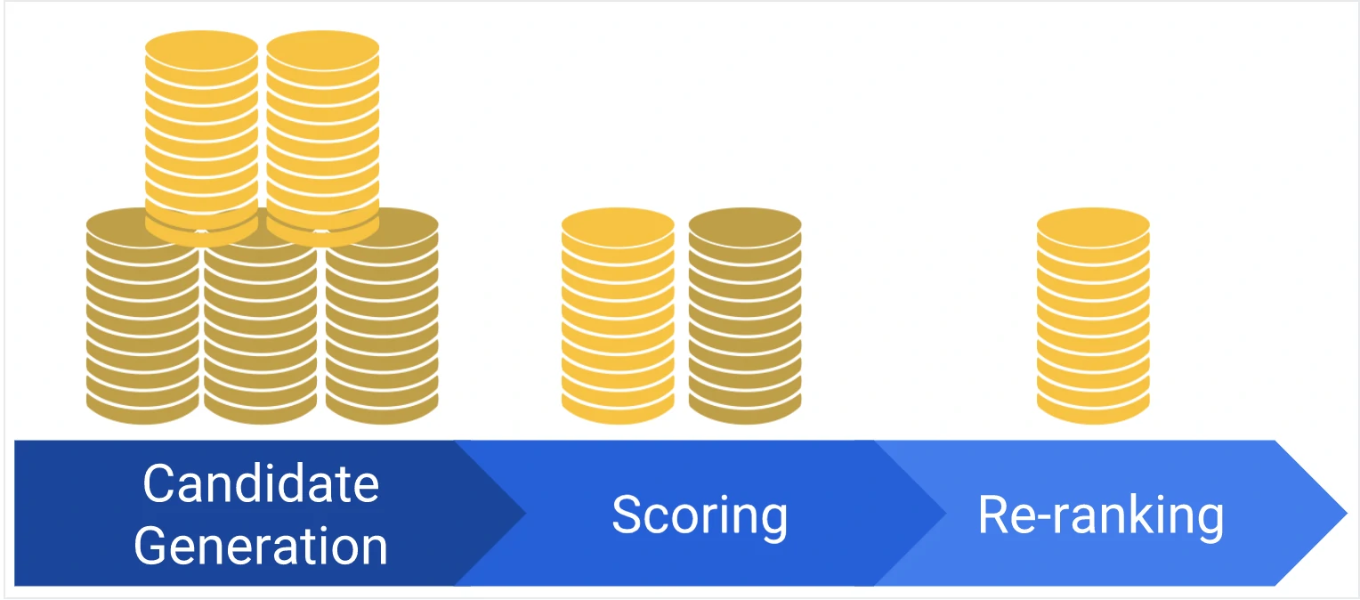
- Candidate Generation: starting with a vast corpus and generating a smaller subset of candidates.
- Scoring: the model ranks the candidates to select a smaller, more refined set of documents.
- Re-ranking: This final step refines the recommendations.
Funnel Architecture
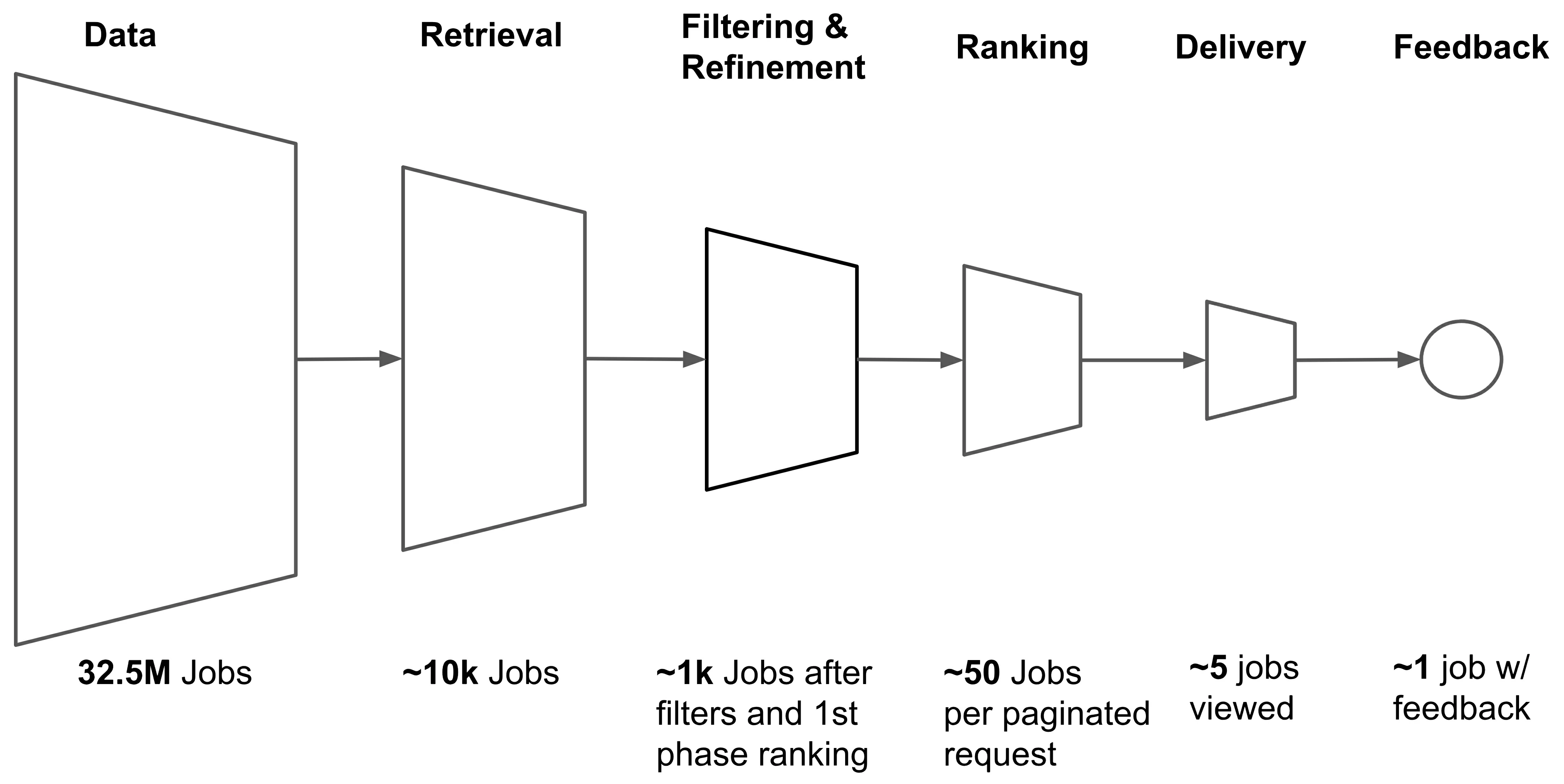
Many large-scale recommendation systems implement these processes in two main stages: retrieval and ranking that wrap up in funnel architecture. Funnel architectures are designed to progressively refine a vast pool of potential candidates into a smaller, more relevant set of recommendations through multiple stages. in example:
- Eugene Yan’s 2-Stage (2x2) Model of a Recommender System
- Nvidia’s 4-Stage (2x4) Model of a Recommender System
2-Stage (2x2) Recommender Systems
The 2-Stage (2x2) model involves two main stages:
- Retrieval: Quickly narrows down the vast candidate pool (e.g., millions of items) to a smaller subset using scalable models such as matrix factorization or two-tower architectures.
- Ranking: Applies sophisticated models incorporating richer feature sets, such as user context or item-specific details, to assign relevance scores and generate a personalized, ranked list.
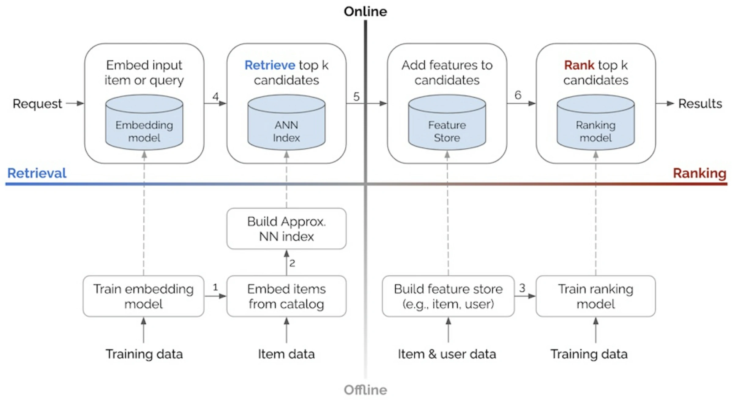
Eugene Yan’s 2x2 model identifies two main dimensions within discovery systems:
- Environment: Offline (flows bottom-up) vs. Online (left-to-right).
- Process: Candidate Retrieval vs. Ranking.
With offline environment, batch processes handle tasks such as model training, creating embeddings for catalog items, and developing structures like approximate nearest neighbors (ANN) indices or knowledge graphs to identify item similarity. The offline stage may also involve loading item and user data into a feature store, which helps augment input data during ranking.
Meanwhile, The online environment serves individual user requests in real-time, utilizing artifacts generated offline (e.g., ANN indices, knowledge graphs, models).
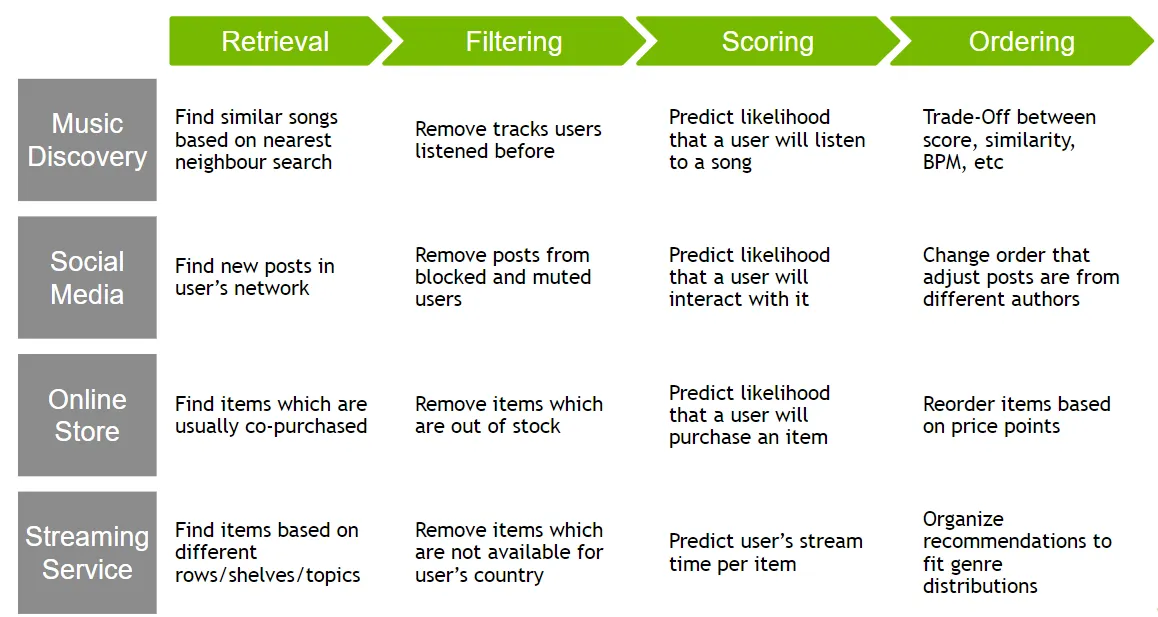
4-Stage (2x4) Recommender Systems
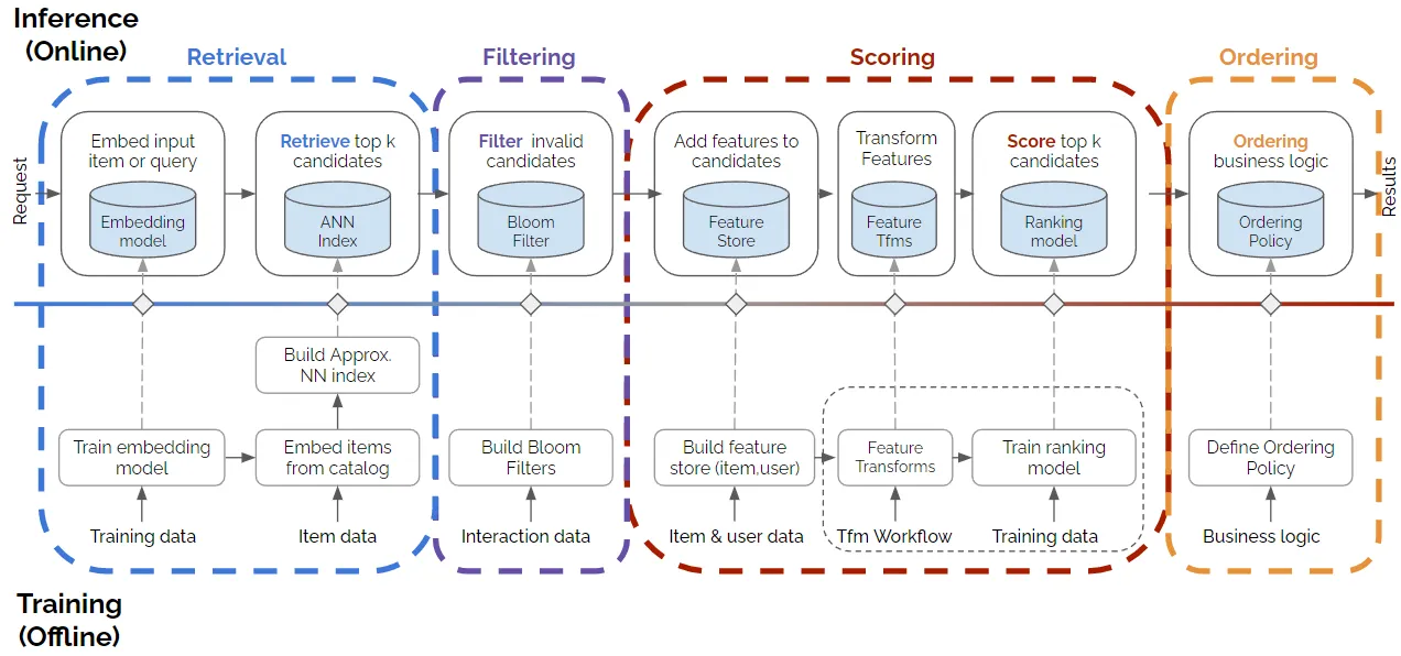
The 4-Stage (2x4) model extends the 2x2 framework with two intermediary stages for greater precision and flexibility:
- Retrieval: Identifies an initial set of candidates, emphasizing efficiency and broad coverage. Using methods such as matrix factorization, two-tower models, or ANN. Retrieval is computationally efficient, ensuring the model can quickly handle a large number of items and narrow them down to a set of potential candidates for scoring.
- Filtering: Applies business rules to exclude ineligible or irrelevant items (e.g., out-of-stock products inappropriate for the user, or regionally restricted content). Filtering ensures that the system does not rely on retrieval or scoring models to handle business-specific logic, allowing for more precise control over item eligibility.
- Scoring: Involves a detailed analysis of the remaining candidates,using models that factor in additional features (e.g., user data, user-item interactions, contextual information) to predict user interest. Scoring can leverage sophisticated models, such as deep learning architectures, to assign interaction likelihoods (e.g., click, purchase probability) to each candidate.
- Ranking (or Ordering): The system arranges items into an ordered list for the user. Although scoring assigns relevance scores to each item, the ordering stage allows further adjustments to ensure a diverse mix of recommendations or to meet additional criteria like novelty and business goals.
These frameworks allow recommender systems to balance computational efficiency in early stages with precision and personalization in later stages. They are widely used in large-scale systems like Netflix, YouTube, and Amazon.
Candidate Generation
- Candidate generation is the first stage of recommendations and is typically achieved by finding features for users that relate to features of the items.
- This step is the process of selecting a set of items that are likely to be recommended to a user. This process is typically performed after user preferences have been collected, and it involves filtering a large set of potential recommendations down to a more manageable number.
- Given a query (user information), the model generates a set of relevant candidates (videos, movies).
- In Example: User searches for computer at some location. It would filter out searches that were not in user’s location and look at latent representation of the user and find items that have latent representations that are close using approximate nearest neighbor algorithms.
- Candidate generation is for recommender systems like a search engine where the candidates are not particularly based on time. whereas candidate retrieval is for news-feed based systems where time is important.
The goal of candidate generation:
- To reduce the number of items that must be evaluated by the system.
- Still ensuring that the most relevant recommendations are included.
Two common candidate generation approaches:
- Content-based filtering: Uses similarity between content to recommend new content.
- Collaborative filtering: Uses similarity between queries (2 or more users) and items (videos, movies) to provide recommendations.
Input Features
This features are broadly categorized into:
- Dense features (Continuous / real / numerical values that directly input into models) such as;
- numerical ratings
- timestamps
- year information
- Sparse features (categorical and can vary in cardinality, that require encoding methods like embeddings) such as;
- categories
- tags
By combining these feature types, models can effectively learn patterns and relationships to generate accurate predictions and recommendations.
Sparse features classified into:
- Univalent Features (single-value)
- features represent attributes with a single value for each entity. These values typically represent a unique attribute or characteristic of the entity.
- Representation using one-hot encoding:
- If a feature can take on n possible categorical values, it is encoded as a vector of size n, where only one position (corresponding to the feature’s value) is set to “1” while the rest are “0”.
- For instance, if there are 5 possible product categories (Electronics, Furniture, Books, Clothing, Food), and a product belongs to the “Books” category, its one-hot vector would look like: [0,0,1,0,0].
- This encoding is sparse but effective for capturing the uniqueness of a single value.
- Example:
device_type ∈ {mobile, desktop, tablet}
device_type device_mobile device_desktop device_tablet mobile 1 0 0 desktop 0 1 0 tablet 0 0 1
- Multivalent Features (multi-value)
- features capture sets of attributes that have multiple values for each entity. These values represent a set of attributes or properties associated with the entity, rather than a single attribute.
- examples:
- categories
- list viewed items
- set of tags
- Representation using multi-hot encoding:
- If a feature can take on n possible categorical values, it is encoded as a vector of size n, where multiple positions corresponding to the feature’s values are set to “1” while the rest remain “0”.
- For example, if a user has watched movies from the genres “Action”, “Comedy”, and “Sci-Fi” out of 5 possible genres, the multi-hot vector might look like: [1,1,0,0,1].
- Like one-hot encoding, this approach results in a sparse representation but can handle sets of attributes effectively.
- Example:
interests ⊆ {sports, tech, finance, travel, gaming}
user_id sports tech finance travel gaming U1 1 1 0 0 0 U2 0 1 1 1 0 U3 1 0 0 1 1
Embedding
Specifically for sparse-multivalent features, it often leads to excessively high-dimensional. Thus we could converted into a low-dimensional, dense real-valued vector, often referred to as an embedding vector.
The embedding vectors are initialized randomly and then the values are trained to minimize the final loss function during model training. The embedding network maps each sparse feature value (e.g., genre or actor) to a low-dimensional dense vector representation called an embedding. These embeddings capture the semantic relationships and similarities between different categories. The embedding lookup tables contain pre-computed embeddings for each sparse feature value, allowing for efficient retrieval during the model’s inference.
Example: Embedding dimension = 4
| interest_id | embedding vector |
|---|---|
| sports | [0.12, 0.81, -0.33, 0.05] |
| tech | [0.44, -0.22, 0.10, 0.67] |
| finance | [-0.31, 0.09, 0.77, -0.18] |
| travel | [0.55, 0.20, -0.40, 0.11] |
| gaming | [0.08, -0.61, 0.35, 0.49] |
Example: Aggregate multiple embeddings (mean pooling)
User U2 interests = {tech, finance, travel}
  tech     = [ 0.44, -0.22,  0.10,  0.67]
  finance  = [-0.31,  0.09,  0.77, -0.18]
  travel   = [ 0.55,  0.20, -0.40,  0.11]

  Mean embedding = [0.23, 0.02, 0.16, 0.20]
These features are typically combined with normalized continuous features (e.g., time since the last event, the number of interactions, or numerical ratings) to form a comprehensive input representation for the machine learning model.
An example of deep learning model architecture for processing both dense and sparse features.
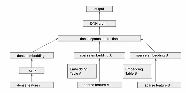
Transforming Variable-Sized Sparse IDs Into Fixed-Width Vectors
At the input stage of the recommendation model, one key challenge is the variability in size of sparse feature inputs. To process these multivalent sparse features efficiently in the deep learning architecture, the following steps are employed:
-
Embedding Sparse Features + Averaging Embeddings First mapped to dense, low-dimensional embedding vectors using embedding lookup tables. Next, transforms the variable-sized “bag” of sparse embeddings into a single fixed-width vector representation.
- Each user has a variable number of IDs:
User A: viewed_products = [P1, P7] User B: viewed_products = [P3, P8, P9, P10] User C: viewed_products = [P2] - Embedding lookup + Pooling (mean, sum, max, Attention-weighted)
User B embeddings:
P3  = [0.1, 0.6, 0.2, 0.0]
P8  = [0.4, 0.1, 0.3, 0.5]
P9  = [0.2, 0.3, 0.1, 0.4]
P10 = [0.3, 0.2, 0.5, 0.1]

# mean pooling, d=4
User B vector = [0.25, 0.30, 0.28, 0.25]
- Each user has a variable number of IDs:
-
Concatenation with Other Features: Concatenated with other feature types, such as dense features (e.g., user age, gender) or other sparse features (that may or may not have undergone similar transformations). This concatenated representation forms a unified, fixed-width input vector that is suitable for feeding into the neural network’s hidden layers.
Benefits of Encoding and Representation
- One-Hot Encoding for Univalent Features:
- Simplifies feature representation for single-value attributes.
- Ensures that each possible category is uniquely represented.
- Multi-Hot Encoding for Multivalent Features:
- Allows effective modeling of sets or groups of attributes without collapsing them into a single value.
- Preserves the full scope of relevant information (e.g., all categories a user interacts with).
Benefits of Averaging embedding
- Dimensionality Reduction: Averaging condenses variable-sized inputs into a consistent format, reducing computational complexity.
- Noise Mitigation: By averaging multiple embeddings, the model can smooth out noise and capture the overall trend or preference represented by the set of sparse IDs.
- Scalability: This approach allows the model to handle a wide range of input sizes without increasing the number of parameters or computational requirements.
Challenges and Considerations
- High Dimensionality:
- Both one-hot and multi-hot encodings can result in high-dimensional sparse vectors, especially when the number of categories is large.
- Embedding Training:
- The quality of embeddings learned from categorical data can significantly impact model performance.
- Interpretability:
- While sparse representations (one-hot and multi-hot) are easy to interpret, embeddings are dense and less transparent, requiring additional techniques to understand their semantics.
Negative Sampling
- The purpose of these techniques is to address bias and dislike items (from users) in the training data and improve the performance and fairness of the models. This is to provide recommendations that are aligned with the user’s interests and preferences, rather than deliberately suggesting items that the user won’t like.
- Negative sampling involves randomly selecting items that the user has not interacted with and assigning them negative labels to represent disinterest or lack of preference (due to we could deduce that un-interaction items could lead to dislike).
- By including negative samples, the model can learn to distinguish between items that a user is likely to prefer and those they are likely to dislike.
- Negative samples are used to help the model learn patterns and make better predictions, but they are not meant to be used as actual recommendations to users.
Evaluation
- The goal of this evaluation is to test if a recommender system has a good candidate generation or candidate retrieval pool.
- Some commonly used metrics are:
- Precision: Precision measures the percentage of relevant items among the recommended items. In the context of candidate generation, precision measures how many of the recommended candidates are actually relevant to the user’s preferences.
- Recall: Recall measures the percentage of relevant items that were recommended. In the context of candidate generation, recall measures how many of the relevant candidates were recommended to the user.
- F1 Score: F1 Score is the harmonic mean of precision and recall. It provides a balance between precision and recall and is a good overall metric for evaluating candidate generation performance.
- Mean Average Precision (mAP): MAP measures the average precision across different queries. In the context of candidate generation, MAP measures the average precision of the recommended candidates across all the users.
- Normalized Discounted Cumulative Gain (NDCG): NDCG measures the relevance of the recommended items by assigning higher scores to items that are more relevant. In the context of candidate generation, NDCG measures how well the recommended candidates are ranked according to their relevance.
Ranking/Scoring
Glosarium
- Embedding: is a learned, low-dimensional dense vector that captures latent semantics.
- Latent representations: is key features of the input data. This could be simplified model of the input data, collection of features that captured by models.